Version 0.0.8 – Rough Draft

Python 3000: Concepts, Turtle = Robot

Loved by beginners and expert programmers alike, Modern Python comes with many built-in modules. Python’s Turtle Graphics Module is one of them.

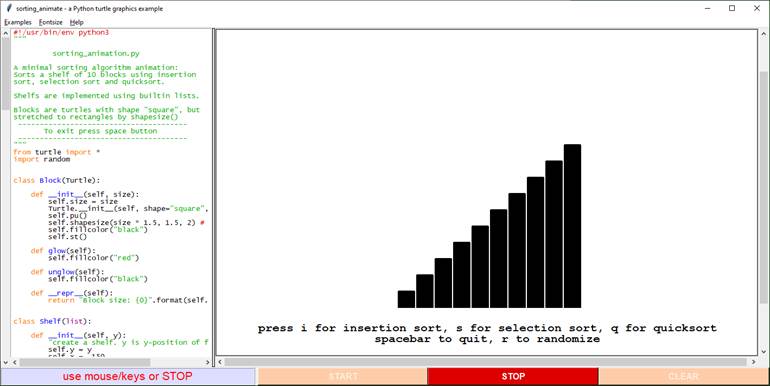
Because Python’s Turtle Graphics Module is built-into many popular Python graphical distributions there is nothing to install.

Training Approach

I have divided all my training into step-by-step modules. Numbered from 1000 to 9000, the numbering system allows us to skip things that we already know to focus upon the things that we do not.

If you are new to programming, then you’ll want to enjoy my free Python Primer.

Prerequisites

To get the most out of Python 3000: Turtles, Robots & Vectors, learners should already know how to create functions, as well as classes, using Python.

If you do not already know how to use Python 3, please complete the Python 1000 series to master functional Python.

If you’ve yet to master Python’s classes and packages, then complete Python 2000 to learn how to use Object Orientation to create classes we can share by creating our own Python Modules. Here are some examples.

Videos are available on Udemy, as well as other educational providers.

If you can use Python classes & functions, then you’ve come to the right place. Be prepared to confidently complete the lessons here!

Python 3000: Turtles, Robots and Vectors

This book is dedicated to showing you how to draw text, grids, polygons, and a variety of shapes using Modern Python. From classic text and lines to Unicode, we’ll even show you how to create a very nice chess board.

We’ll begin by reviewing common graphical concepts. From Cartesian planes & plotting to the computer’s “Purely Positive Plane,” we’ll discuss how using Python’s Turtle Graphics Module can use a combination of several plotting strategies.

You’ll next discover how to draw shapes, pictures, stamps & images, as well as textual glyphs.

Upon completing this training you will understand how to create amazing drawings using the classic Cartesian point-plotting system, the classic Computer plotting system, and – of course – Python’s Turtle Graphics location-relative (“move to, draw to, go to”) way of using “turtle robots” to draw a surprisingly huge number of shapes.

Python 3000: Part One, Points & Vectors – The Big Ideas

So welcome to Python 3000! Your perfect place for Pythoneers who know the difference between Python’s functions, classes, and modules.

A Classic Cartesian Plane

By way of review, in modern mathematics what we are first taught when starting Geometry is how to work with a “Cartesian Plane.”

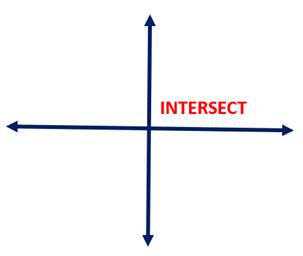
Figure 1: Line Intersection

Initially explored in “two dimensional” terms, the Cartesian Plane has two intersecting lines. One of those lines manages numbered points sitting across the horizon, spaced left to right. The other line manages points spaced up and down an intersecting vertical line.

Of course, when we're moving across the horizon, we're moving either positively or negatively across the x line, or x axis.

When we're moving up and down vertically, we're moving either positively or negatively along the y line, or y axis.

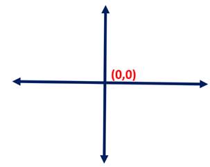
Figure 2: Intersection Point

The point where these two lines intersect on the screen is where both the x and the y location equal zero. Ihe intersection point, as shared in Figure 2, I like to think of as “Point Zero.” The center of our galaxy?

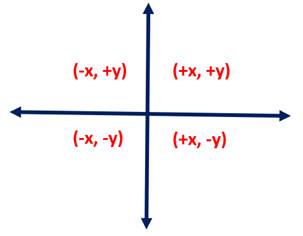
Figure 3: Cartesian's The Four Planes

Classically there are no more than 360 directions to move away from wherever we are, or 360 Degrees.

All powerful concepts, Point Zero also divides the Cartesian galaxy into four regions. Each a uniquely navigable area, there is but a single “purely positive” region, a “purely negative,” as well as each for two positive:negative complements as seen in Figure 3, above.

The first truth table?

Cartesian graphics is all about locating x, y intersections, or points, within its four different areas.

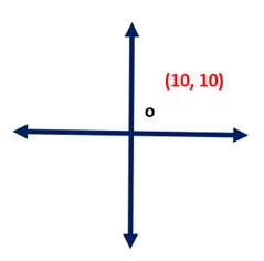
Figure 4: Cartesian's 'All-Positive' Plotting Area

So if setting both x and y equal to 0 will take us to “Point Zero,” if we were to set both x and y equal to 10 we’d arrive at what we might call “Point 10,” as plotted in Figure 4, above.

Interestingly, the computer’s default drawing system is completely different.

The Classic Computer Plane

Decidedly not Cartesian, in every computer language that I've ever used the classic computer’s zero-point origin is not located in the middle of four planes, but in the upper left-hand corner of a single plotting plane:

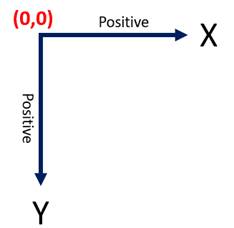
Figure 5: Classic Computer Plane

On computers we’ll most often find ourselves forever plotting points in the positive as we see in Figure 6, below.

Contrasting the Cartesian experience in Figure 3 with the default classic plotting system in Figure 4 (above) we can begin to understand the difference between the Cartesian, and the Computerized, point plotting paradigms. While the ideas of having an origin, horizontal, and vertical line are similar, notice how Point 10 falls below, rather than above, Point Zero:

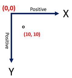
Figure 6: Positive Computer Point Location

Having but a single purely positive point coordinate system, limited to a single plane, makes finding locations easier for the computer. -But sometimes having but a single, positively numbered plane also makes statistical modeling very difficult for those equations used to plotting their results into Cartesian’s four plotting areas.

Multiple Turtles

Easy enough.

But consider the power of having more than one Turtle?

From game play to real-world artificial intelligence, being able to define multiple objects, each operating around their own origins & homes, makes programming classes much easier.

The concepts we learn when using Turtle Graphics also allows everyone to discuss missions objectively, certainly when we’ve many objects running around at once.

Turtle Backstory

Tuttle Graphics was conceived in the 1960s by Seymour Papert.

Papert likened the plotting system to a Turtle walking across a plane, its tail dipped in ink.

Yet because the visualization is extremely easy to understand, whenever we say we are using Turtle Graphics, some may sneer?

For our part we should focus on the enlightened idea that Turtle Graphics can manage entire armies of turtles. Simply calling the “turtle” an “object,” or a “robot,” eliminates ridicule.

Indeed, the concept of modern Turtle Graphics is so respected to have implementations not only in Python, but available Logo, Java, as well as many other programming languages as well.

The journey of a million robots begins with a simple way to manage any single Turtle.

Python 3000: Part One, Robotic Turtles – Lesson 1

So let’s get coding.

Module -v- Class

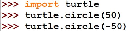
Because we can use it to draw, we often think of the turtle module as being the “default turtle:”

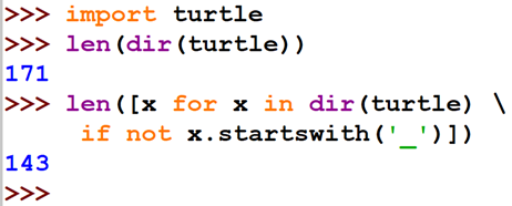
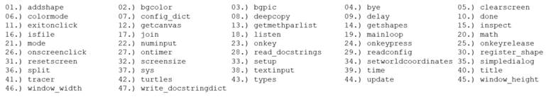
The turtle module has a lot of public members – over 140:

Interestingly, in addition to the module, we’ve the Turtle() class:

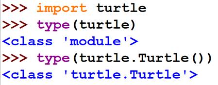
The module & class share documentation & drawing operations:

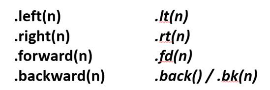
Table 1: Common Robotic Operations

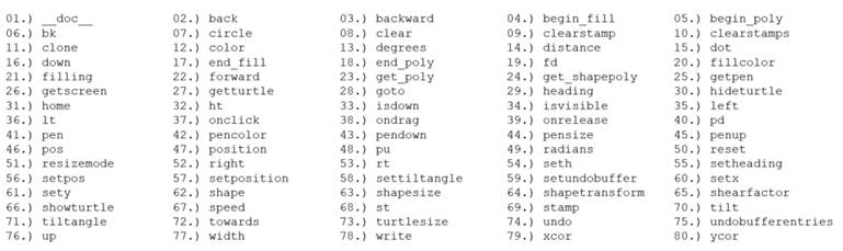
Thus we can use either the Turtle Module proper, or an instance of turtle.Turtle(), to interactively draw upon our screen:

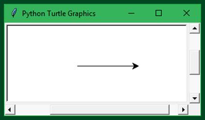
Figure 7: The  X Ray

Your Robot’s Default Location

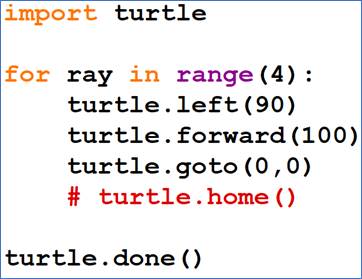
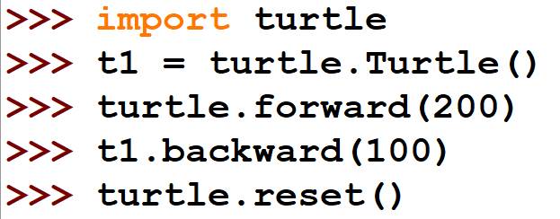
In Figure 8 (above) we're going to access the forward member function of the ‘default turtle’ to advance your Turtle instance ahead 100-pixel elements across your screen:

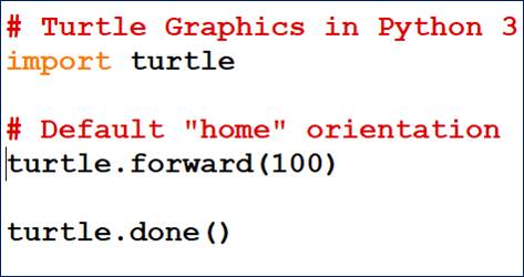
Source 1: Forward & Done

As you may expect, the default location for our default turtle will be in the center of that Cartesian plane, or coordinate (0,0).

What may be unexpected is that when we access the default plane, every robot will be facing in a positive direction – positioned to move across the x axis. It’s tail (or pen) down, dipped in ink, and ready to draw.

What also might be unexpected is that the turtle will set focus to its drawing window upon executing the default turtle’s .done() operation. We’ll return back to the interactive mode only after that drawing window has closed, or after we're .done().

WARNING: Once the default turtle instance is .done() the best practice is to CLOSE THE WINDOW before using that turtle again!

The Way of the GUI

Are you one of the few able to challenge themselves? Take a moment to stop & enjoy a new idea?

I would challenge you now to go ahead and open your Python of choice to input the above simple, three-line program. Be sure to use a graphical user interface.

Verify not only that are you using Python 3, but that you are able to see something like what we see in Figure 8. (your colors may vary!)

Default Home Locations

Whenever we need to jump an Object back to where it came from, we can use the Turtle’s .home() member function.

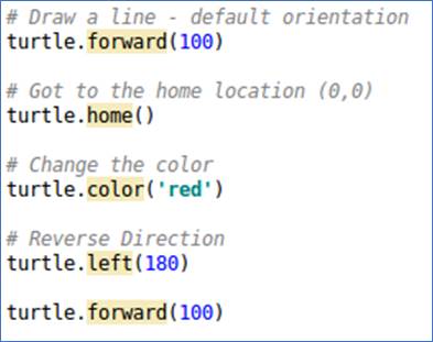
Source 2: Using .home()

And of course, we can also change colors - as we see here to red - as well as to move in many different directions.

So rather than using a negative coordinate system - which is also possible - we can rely upon the object’s default direction.

See if you can use your turtle’s .left(90) to create the following:

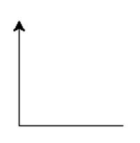
Figure 8: Right Angle & Ray

Feel free to take a moment to complete this activity to practice moving self-relative to whatever direction our Object / robot wakes up in. After your program has run your screen should look pretty much like you saw in Figure 8, above.

Python 3000: Part One, Vector Basics - Lesson 2

There is more than one solution to the previous activity.

Our solution to was saved to the LAB_RightAngle.py file:

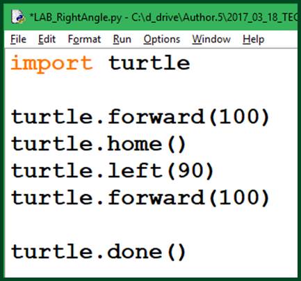
Source 3: Right Angle & Ray

The solution can also be found in the resources associated with this training.

.home()

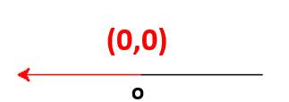
Notice that we’re moving our Turtle - Object to another location when using .home():

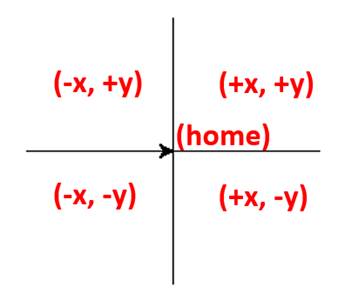
Figure 9: Home Restores Default Direction

By using .home() we're also restoring our default direction, as well.

In addition us a .right(degrees), you may suspect that we’ll have many more functions we can use in addition to the .left(degrees), as well.

.goto(x,y)

Rather than using .home(), we can instead choose to use the Turtle’s .goto() operation.

Source 4: Goto Four

Unlike when using .home(), choosing to use the Turtle’s .goto(0,0) member function preserves our object’s direction. We can also use .setposition().

Convenience Functions

Any turtle has the ability to go forward as well as backward. Once again specifying the number of pixels to be moved, but more importantly each one of these movement member functions also have a “convenience” or an “alias” function:

For our next activity let's go ahead and apply what we've seen and have a little challenge to create our Cartesian Cross:

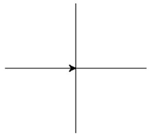
Figure 10: Turtles Cartesian Cross

And once again seeing our default robot shape on the screen above. We’ll see how to change the shape of the robot later on.

Go ahead and take a moment to create your own Cartesian Cross.

Python 3000: Part One, Shapes 360 - Lesson 3

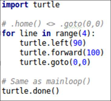
Now we understand that if we were to use .home rather than .goto that we'd restore our default orientation:

Source 5: LAB_Cartesian.py

Feel free to run Source 5 both with & without the comment. Verify that all we're doing when we go home is to have our default orientation restored. -Because how we chose to draw our lines, nothing really happens when we decide to use .home rather than the .goto operation, so you’ll have to add new code.

Turtle Hoards

We’ve seen that there are many member operations that can be shared between different Turtle instances. Note, however, that the default Turtle instance – or the module turtle - has some unique properties the other turtles cannot use:

Table 2: Unique Module Operations

.resetscreen() & .clearscreen()

Every artist knows that the more the mistakes, the greater the mastery?

Try this at home:

No matter if we’re in interactive or non, .reset() sends us .home(), as well removes what we’ve done with any single turtle.

To prove that the default turtle has returned to Point Zero:

We can also clear the entire screen – removing everything – simply by entering:

(#5 in Table 2, above.)

Screen State Challenge

We were able to verify that the .home() and .reset() operations restored an object’s start-state by moving the robot after each.

Verify that operation #5 in Table 2, and #8 in Table 1, works as you might expect.

See help(clearscreen) for more information.

Finally, verify the difference between .reset() and .resetscreen(), as well.

Titles & Window Sizes

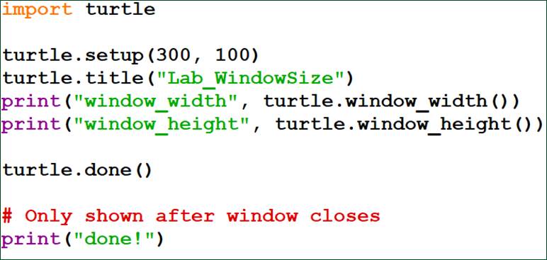
Another one of those unique member functions is the .setup member function, #33:

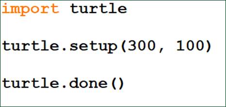
Source 6: Window Size = 300 x 100

Obviously powerful, the default turtle.setup() operation allows us to set up or change the size of our window. For example, we can have a specific width and height for the main window.

Because turtle.setup has defaulted parameters, we could also specify screen sizes in floating-point percentages, adding desktop x & y locations as optional 3^rd and 4^th parameters, respectively:

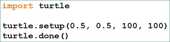
Source 7: Size as Percentages & Desktop Location

You may imagine we also are able to look at our window’s width height (#45), as well as many other window related properties. Each & all unique to the default Turtle.

REPL 1: Default Turtle Ops

To prove that what we have is unique to our default turtle, simply instance another turtle, then try to access these exact same operations.

REPL 2: Instanced Turtle Exceptions

We will see that we will indeed have an exception, in this case specifying that the instance of Turtle does not have an attribute that manages window attributes.

Window Titles

Whenever we want to have a custom title for our application - which of course is going to be most of the time – the default Turtle also has a member function. Using turtle.title() will allow us to set the window’s title to any Unicode string that we may wish to see:

Source 8: Titles & Cleanup Operations

For our next activity let's go ahead and have a little fun to simply try what we've seen.

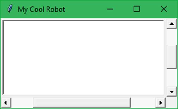
Figure 11: A Custom Solution

Your solution need not look like what we’ve provided in the Source 8 example, above.

Python 3000: Part Two, Vectoring – Lesson 4

Well now that we have our bearings let's take a moment and start drawing some interesting things with lines. Specifically let's talk about using grids and polygons.

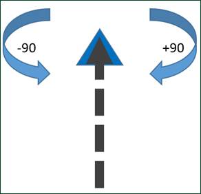
Figure 12: Positive & Negative Rotation

If you look at the tip of the arrow in Figure 13, you can imagine that in order to get to a certain place that your Turtle has to come from an area then move toward wherever we’ve pointed it.

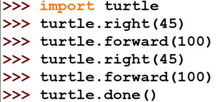
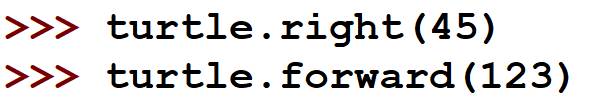
REPL 3: Where We're Heading

Once pointed, if we decide to pivot to the right by 45 degrees we would say “rotate right, positive 45 degrees” before moving. Pivoting twice results in rotating 90 degrees:

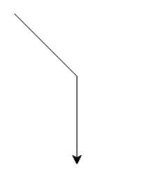
Figure 13: 45 + 45 = 90 Degrees

Of course, if we wanted to go to the left we would simply say that we wanted to “rotate left, negative 45 degrees” to create Figure 14 once again.

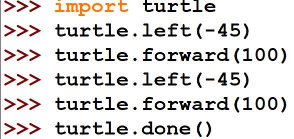
REPL 4: Same Results!

Using what you know now, now try to draw:

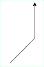
Figure 14: Left Positive, or Right Negative

Go ahead to re-create Figure 15. Take a moment to do that now.

Mixed Instances

Re-creating Figure 15 was easy, so we decided to show how to mix things up a little to demonstrate a few more concepts:

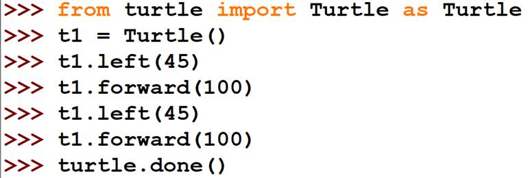
REPL 5: Two Instances

In addition importing turtle.Turtle as simply Turtle, REPL 5 demonstrates - even though we created our own as t1 – that we still had to use turtle.done(), so we’ll still have to destroy the window when we’re done.

Python 3000: Part Two, Closed Shapes – Lesson 5

Drawing closed shapes is often simply a matter of starting and finishing up in the same place.

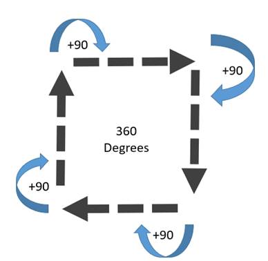
Figure 15: 360 Degrees

Keeping that round-trip in mind, draw the following:

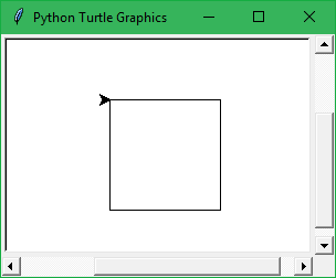
Challenge 1: Draw The Square

Because all we had to do was combine what we gleaned from Figure 16, going right 90 degrees, four times, would complete the assignment.

Here is our solution:

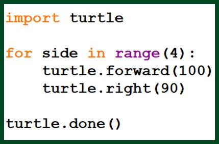
Source 9: LAB_Square.py

And as you can see in Source 9, leveraging Python’s built in range() function allowed us to repeat the `for` block for a total of “zero to three” iterations, drawing a total of four sides.

Source 9 is but one of many solutions. I'd be very surprised if even your variable names were the same?

The Octagon Challenge

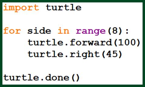
When drawing four sides was easy, how about drawing eight?

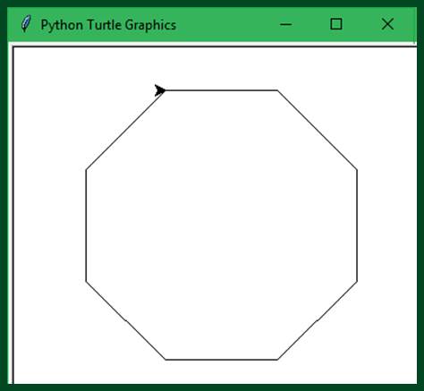
Challenge 2: The Oct Box

As you might imagine we're still going to have 360 degrees, yet rather than divided by 4 to give us 90, we're going to now divide it by 8 to give us the 8-angle result.

So go ahead and challenge yourself and see if you can update your previous solution to draw an octagon “your way”.

Easy Octagons

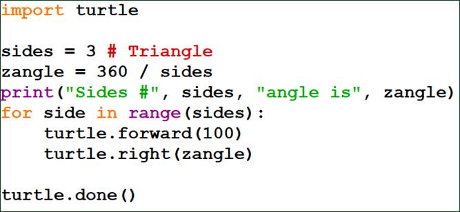
The notion of having 360 degrees, divided by the number of sides that we wish to have in our polygon, works well:

Source 10: My Oct Box

We now have a formula that we can use to create a function that we can call simply by specifying the number of sides to draw the desired polygon.

Try the following:

Equation 1: Testing The Triangle

Challenger: Weaponize the Formula!

A decent research activity, Equation 1 (above) points us to what we should probably next do. Our challenge is to provide a function that we can re-use to complete:

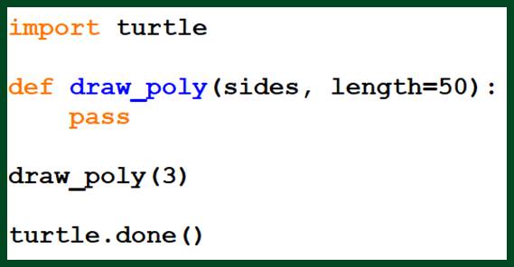
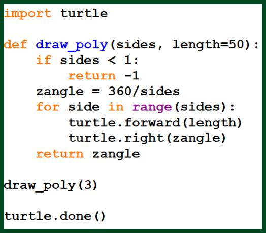
Challenge 3: draw_poly()

While we use the default value of 3 to draw a triangle, note the default length parameter of 50.

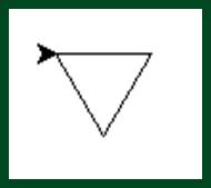
Figure 16: Three sides, default length of 50

And as we've seen in our Python 1000, creating a function with defaults allows us to always have – in this case - unified line lengths. The length parameter can be overridden to allow us to also have custom lengths.

So your challenge is to take a moment and provide an implementation to our draw_poly that allows both a different, as well as a custom, line length.

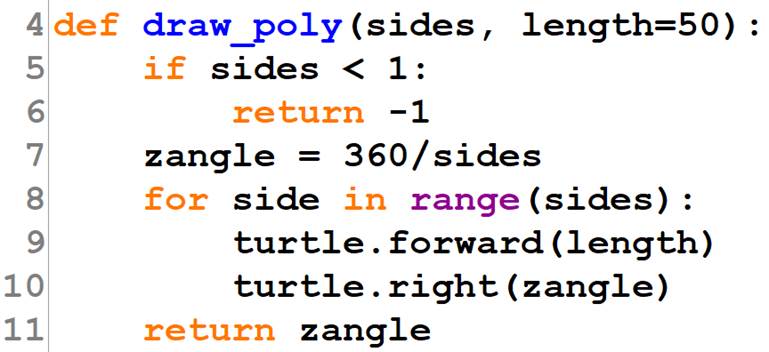
Our draw_poly Soluton

Notice in Source 11 (below) that our solution had a little bit of sanity checking? Specifically, if you wanted to know if the sides were less than one, we returned -1 as the result. In the future we could also return -1 if something else failed to work.

To tell us that the drawing went as planned, even though we didn't originally require a result to be returned, we decided to return the calculated angle as the result. It is always nice to know if all went well:

Source 11: LAB_draw_poly.py

We also copied the code from Equation 1.

Python 3000: Part Two, Grid of Grids – Lesson 6

Now that we’ve a function we should talk about other opportunities to reuse draw_polly.

Let's take a moment to see how we might be able to use vector-based graphics to draw a grid:

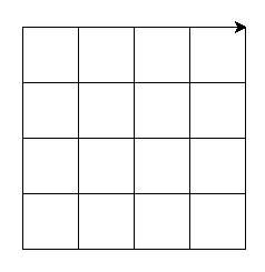
Figure 17: The Grid Problem

Code Re-Use

To draw the grid the first thing that we can now do, of course, is to simply include and re-use our draw_poly algorithm.

Source 12: Reusing draw_poly

Rather than 360/3, we're going to have 4 sides to our polygon. Easy enough to understand.

Default Parameters

Even though the length of 50 is the same as the default parameter value, coding a line length on line 23 allows us to play with other values:

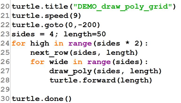
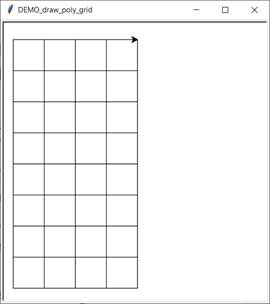
Source 13: DEMO_draw_poly_grid.py

Controlling Drawing Speed

Setting the speed to 9 on line 21 above allows us to observe the drawing operation.

Line 24 controls grid height. Rather than 4, we decided to use 4 * 2 = 8 rows.

The next_row function on line 13 is where we move the “robot” around:

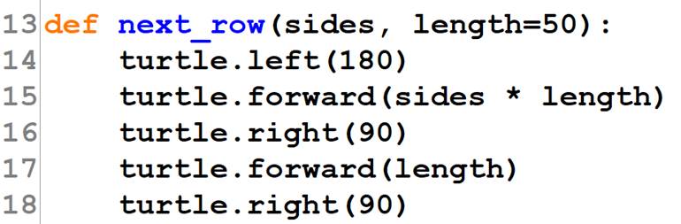
Source 14: Grid Turtle Placement

The Grid Super Challenge!

The toughest problem we’ve yet encountered in Python 3000, see if you can challenge yourself to create a customizable “square of squares” to create a grid.

Using a grid to exactly track what we're doing is a very useful capability to have. The ability to draw a grid should be part of our standard toolkit:

Challenge 4: Grid of Grids

Python 3000: Part Two, Serpentine Grids – Lesson 7

Faster Grids

While Challenge 4 is arguably a very good object-oriented solution, drawing that square over and repeatedly isn’t very efficient.

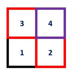
Figure 18: Overlapping Shapes

A faster way, of course, would be to eliminate the overlap.

The Serpentine Grid Challenge

One efficient grid strategy could be more serpentine: moving back and forth both horizontally, as well as vertically?

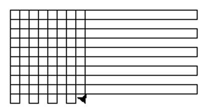
Figure 19: Serpentine Grid Strategy

Another challenging activity, your next mission – if you decide to accept it – is to draw a “serpentine grid.”

A Serpentine Grid Solution

My solution for the “Figure 20 Challenge” is in the resources as DEMO_serpent_grid.py.

Python 3000: Part Two, Grid Class – Lesson 8

Here is the source for DEMO_serpent_grid.py:

import turtle

def draw_grid(zturtle, width, height, cell_size, border=None, border_pen_size=None):

    ylines = int(height / cell_size)

    xlines = int(width / cell_size)

# y serpentines

    zturtle.home()

    next_angle = -90

for yy in range(xlines):

        zturtle.forward(height)

        next_angle = next_angle * -1

        zturtle.right(next_angle)

        zturtle.forward(cell_size)

        zturtle.right(next_angle)

# x serpentines

    zturtle.home()

    next_angle = 90

    zturtle.right(next_angle)

for xx in range(ylines):

        zturtle.forward(width)

        next_angle = next_angle * -1

        zturtle.right(next_angle)

        zturtle.forward(cell_size)

        zturtle.right(next_angle)

# Outer Box

    zturtle.home()

if border:

        zturtle.color(border)

if border_pen_size:

        zturtle.pensize(border_pen_size)

    zturtle.pen(10)

    zturtle.right(90)

    zturtle.forward(width)

    zturtle.right(-90)

    zturtle.forward(height)

    zturtle.right(-90)

    zturtle.forward(width)

    zturtle.right(-90)

    zturtle.forward(height)

    zturtle.home()

if __name__ == "__main__":

    draw_grid(turtle, 100, 200, 10, border='green', border_pen_size=3)

Our solution above added an outside border. We did not use dry_poly, but copied the concept.

We're going to be slithering like a serpent and by moving to the next and then forward our ourselves and moving back again back and forth across our screen. First horizontally – across the x axis, then vertically across the y.

Refactoring Challenge: SnakeGrid

Complicated enough to study, a great way to make the code easier to understand would be to refactor draw_grid into a class.

Here is the requirement:

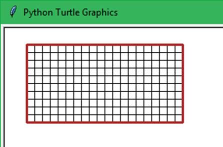
Figure 20: Serpentine Class Grid

Feel free to create a static class:

class SnakeGrid:

@staticmethod

def draw_rectangle(zturtle, x, y, width, height, border=None, border_pen_size=None): ...

@staticmethod

def draw_snake(zturtle, x, y, height, cell_size, xlines, next_angle): ...

@staticmethod

def draw_grid(zturtle, x, y, width, height, cell_size, border=None, border_pen_size=None): ...

As you can imagine we are going to use the same logic as seen in the draw_grid.

Serpentine Class Solution

Located in LAB_SerpentClass.py, to better compare the two techniques we decided to create two classes. Class SlowGrid demonstrates the slower overlapping approach. Class SnakeGrid, our requirement.

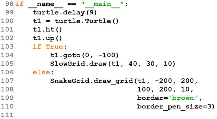
Figure 21: Slow -v- Fast Grid

Reviewing our solution’s main ‘driver’ in Figure 21, line 101 hides the t1 Turtle, then line 102 raises its pen. Once the pen is up, t1 can .goto wherever it needs to without leaving a line behind.

Line 103 permits us to choose which class we’d like to see.

Locate and run LAB_SerpentClass.py, feeling free to change both the speed, as well as line 103, to see how fast / slow either of these strategies can be.

Python 3000: Part Three, Stateful Object – Lesson 9

The rest of this tome remains a work in progress. Until it is done, you can complete this course online.